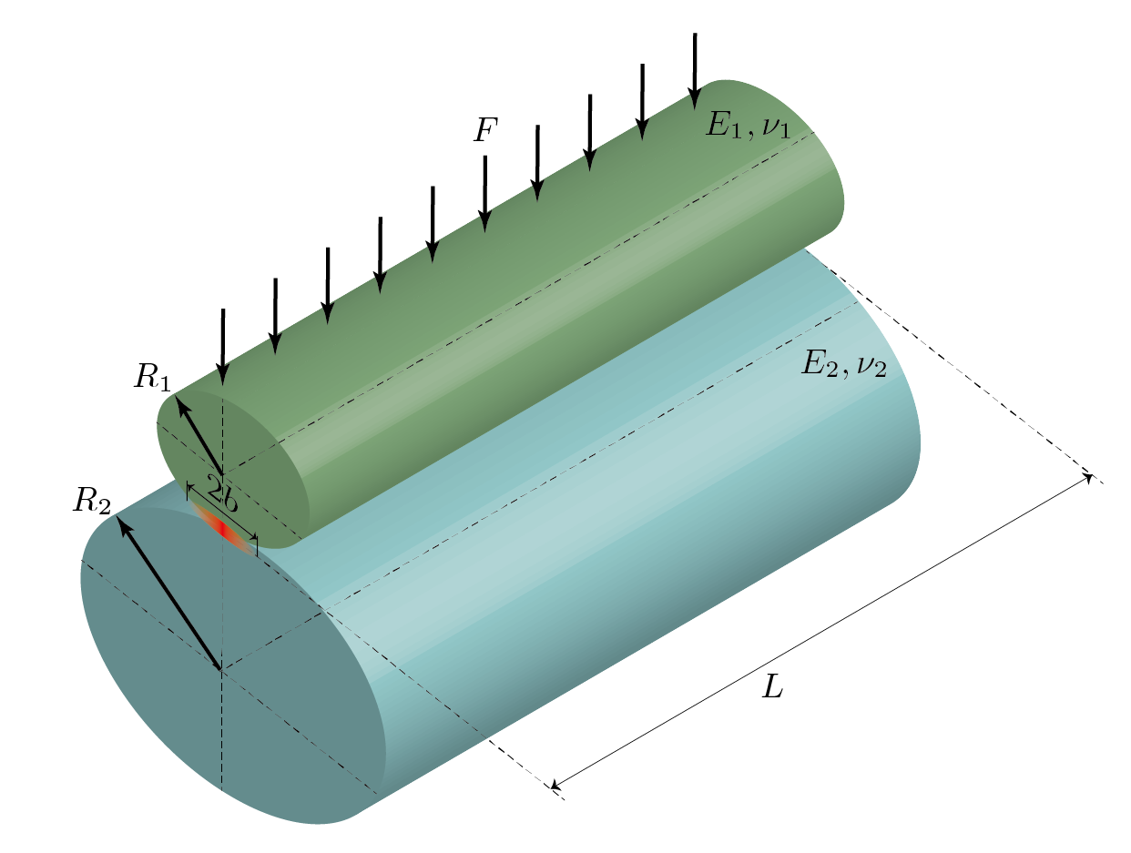
As Pereira said "Only the Johson and the Radzimovsky models are
suitable to describe the contact involving colliding cylinders in most
of practical applications."
% initial value for fit
n = 10/9;
k0 = 1e10;
n0 = 1;
% fitfun1(): k is unknown
fitfun1 = @(k,delta) k.*delta.^n; % n = 9/10
% fitfun2(): k and n are unknown
fitfun2 = @(para,delta) para(1).*delta.^para(2); % para is established for nlinfit()


% fit for Radzimovasky model
% fitfun1
[kRadzi1, ~,~,~,MSERadzi1,~] = nlinfit(deltaRadzi, F, fitfun1, k0);
% fitfun2
[fitParaResult, ~,~,~,MSERadzi2,~] = nlinfit(deltaRadzi, F, fitfun2, [k0, n0]);
kRadzi2 = fitParaResult(1);
nRadzi2 = fitParaResult(2);
% plot for Radzimovasky model
plot(deltaRadzi,F,...
     "LineWidth",2); hold on
plot(deltaRadzi,fitfun1(kRadzi1,deltaRadzi),...
     'o',...
     'MarkerIndices', 1:num/20:num); hold on
plot(deltaRadzi,fitfun2([kRadzi2,nRadzi2],deltaRadzi),...
     's',...
     'MarkerIndices', 1:num/20:num); hold off
xlabel('$\delta$ (m)','Interpreter',"latex")
ylabel('$F$ (N)','Interpreter',"latex")
title('Line Contact - Fit Model - Radzimovasky')
legend( 'Radzimovasky model',...
        '$F = k_{Hertz} \delta^{10/9}$',...
        '$F = k_{Hertz} \delta^n$',...
        'Interpreter',"latex",...
        "Location","best")
1
2
3
4
5
6
7
8
% print fit result
fprintf(['       k unknow  k and n unknow\n' ...
         'n      %6.6f  %6.6f\n'...
         'KHertz %6.2e  %6.2e\n'...
         'MSE    %6.2e  %6.2e'],...
         n, nRadzi2,...
         kRadzi1, kRadzi2,...
         MSERadzi1, MSERadzi2);
% fit for Johnson model
% fitfun1
[kJohnson1, ~,~,~,MSEJohnson1,~] = nlinfit(deltaJohnson, F, fitfun1, k0);
% fitfun2
[fitParaResult, ~,~,~,MSEJohnson2,~] = nlinfit(deltaJohnson, F, fitfun2, [k0, n0]);
kJohnson2 = fitParaResult(1);
nJohnson2 = fitParaResult(2);
% plot for Radzimovasky model
plot(deltaJohnson,F,...
     "LineWidth",2); hold on
plot(deltaJohnson,fitfun1(kJohnson1,deltaJohnson),...
     'o',...
     'MarkerIndices', 1:num/20:num); hold on
plot(deltaJohnson,fitfun2([kJohnson2,nJohnson2],deltaJohnson),...
     's',...
     'MarkerIndices', 1:num/20:num); hold off
xlabel('$\delta$ (m)','Interpreter',"latex")
ylabel('$F$ (N)','Interpreter',"latex")
title('Line Contact - Fit Model - Johnson')
legend( 'Johnson model',...
        '$F = k_{Hertz} \delta^{10/9}$',...
        '$F = k_{Hertz} \delta^n$',...
        'Interpreter',"latex",...
        "Location","best")
1
2
3
4
5
6
7
8
% print fit result
fprintf(['       k unknow  k and n unknow\n' ...
         'n      %6.6f  %6.6f\n'...
         'KHertz %6.2e  %6.2e\n'...
         'MSE    %6.2e  %6.2e'],...
         n, nJohnson2,...
         kJohnson1, kJohnson2,...
         MSEJohnson1, MSEJohnson2);
Output:
k unknow
k and n unknow
n
1.111111
1.160895
KHertz
3.94e+09
5.80e+09
MSE
7.10e+07
1.72e+06
Reference
Hale, Layton C. Appendix C: Contact Mechanics, in "Principles and
techniques for desiging precision machines." MIT PhD Thesis, 1999. pp.
417-426.
K. L. Johnson, “Non-Hertzian normal contact of elastic bodies,” in
Contact Mechanics, Cambridge: Cambridge University Press, 1985, pp.
107–152.
A. C. Fischer-Cripps, "Elastic Contact," In Introduction to Contact
Mechanics. Mechanical Engineering Series, Boston: Springer, 2007, pp.
101-114.
Cândida M. Pereira, Amílcar L. Ramalho, Jorge A. Ambrósio. A
critical overview of internal and external cylinder contact force
models. Nonlinear Dynamics, 2010, 63 (4), pp.681-697.
Some slids in web:
https://my.mech.utah.edu/~me7960/lectures/Topic2-FundamentalsOfErrors.pdf